Critical Considerations in Process Safety

Understanding the desired reaction

Here, the key pieces of information to extract are:

• What is the energy evolved in the reaction?
• What is the cooling capacity required in the manufacturing plant to maintain an isothermal reaction?
• What is the subsequent rise in temperature when no cooling is applied?

Chemical reactions involve the transformation of reactants into products; heat will be exchanged with the environment in the process. In the case of exothermic reactions, energy will be released, and if the reaction is endothermic, energy will be absorbed. Understanding the thermodynamic nature of this transformation is fundamental. If endothermic and external energy is not supplied, the progression of the reaction can be very slow, making it inefficient. But on the other hand, if a chemical process is exothermic, associated risks might come, such as high temperature or high pressures.

Calorimeters can be used to perform the characterization of the chemical reaction. If the temperature is to be kept constant in the reaction (isothermal conditions), energy needs to be supplied to maintain this condition. This would tell us how much energy the reaction produces or takes. These energy values scale linearly, so we can calculate the energy required for the industrial scale using the value obtained from the calorimeter in a small-scale experiment.

As an example, we can use the esterification of acetic anhydride with methanol, which produces ethyl acetate and acetic acid:

(CH₃CO)₂O + CH₃OH → CH₃COOCH₃ + CH₃COOH

This is an exothermic reaction that releases 66 kJ mol^-1. A calorimeter, like a Simular can be used. In this case, we can use a semi-batch regime, adding the reactant (acetic anhydride) at a feed rate of 2 g·min^-1 over 50 mins and keeping the temperature at 30°C. As the reaction progresses, heat is released, and the cooling system activates to maintain a constant temperature. The figure below shows the power supplied to the reactor to keep the reaction isothermal (in W), how much acetic anhydride has been supplied (in g), and the energy released (in J).

In the following example of a semi-batch esterification reaction process, acetic anhydride was added at a 2 g/minute dosing rate over 50 minutes to methanol in a 1 L reactor in the Simular reaction calorimeter. At the same time, the temperature was held isothermally at 30°C [1]. Figure 5 shows the:

• Reaction power (this is essentially the rate of heat generation) [pink trace]
• Energy released [blue trace]
• Feed rate [yellow trace]

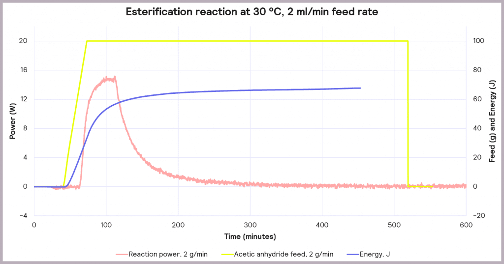
Under these conditions, it can be seen that the reaction power reaches a maximum of 15W.  This means a cooling capacity of at least 15 W is required to keep this reaction isothermal.  As a first check, these values can be proportionately scaled up: for example, the reaction was performed in a 1 L reactor, so for a 2000 L pilot reactor, this would indicate that at least a 30 kW (30,000 W) cooling capacity is required for the larger system.

Also, the measured value for the energy released during the reaction is around 66 J, which progresses even when the reactor feed has finished. The energy released after the feed stopped is 34.6 kJ. This allows us to know the maximum temperature of synthesis reactions using the following equation:

Where T_p is the temperature of the reactor (in this case, 30°C) and ∆𝑇𝑎𝑑,𝑥 is the adiabatic temperature increase. This is the change in the temperature when there is no heat exchange with the surroundings – so it just comes from the reaction itself. These values can be calculated using another equation:

Where mC_p is the thermal mass of the components (the mass multiplied by the heat capacity), and its value is 326 J°C^-1. This means that the adiabatic temperature increase in the reactor is 106°C, so the total MTSR is 136°C. ∆𝑇𝑎𝑑,𝑥

Thus, reaction calorimetry enables the heat evolved during the desired reaction to be measured, which is then used to calculate the cooling capacity required to keep the system at the desired reaction temperature – T_p.

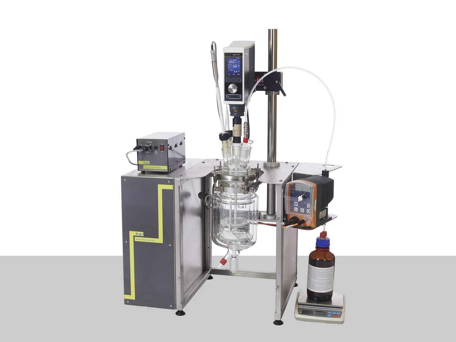
Simular | Process Development Reaction Calorimeter

This highly configurable system from the H.E.L product family excels in optimizing process...

Details

Identifying and understanding decomposition and secondary thermal runaway (the undesired reactions)

The use of calorimetry can help us characterize our target chemical reactions: power required to maintain isothermal conditions, runway reactions when cooling is not supplied, and what maximum temperature the reactor can reach.

However, additional reactions may occur in many cases when some of the reagents or products can undergo subsequent chemical reactions. The velocity of these side reactions can exponentially increase when the temperature rises due to the progression of the desired reactions. Among these side reactions, decomposition reactions are of special relevance. Decomposition reactions are those chemical reactions in which one reactant breaks down into two or more products.

A secondary thermal runaway is likely to occur if MTSR is greater than the onset temperature of a component in the reaction mix (T_d). The onset temperature can be defined as the temperature at which the decomposition reaction starts to be detected. This scenario is illustrated in Figure 6.

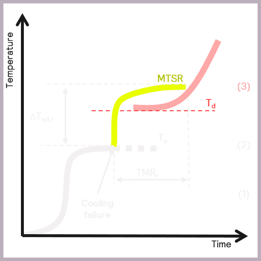
As previously described, MTSR is estimated from reaction calorimetry, while the onset temperatures of materials are determined using thermal screening tools, such as the Thermal Screening Unit (TSu).

A more accurate value of the onset temperature can be determined using adiabatic calorimetry. Still, it is often considered sufficient to use a more straightforward thermal screening tool at this stage. The TSu enables representative samples of the reaction mix to be screened and reliable onset temperatures determined for the reaction intermediates and products. Thermal stability studies also need to take place on the reaction waste stream, which the TSu also facilitates with isothermal stability screening. Just as it is important to identify hazards during the reaction itself, it is also important to understand if there are any longer-term stability issues in the waste products formed so that these issues can also be mitigated.

Suppose it becomes apparent that there is a risk of a secondary thermal runaway occurring. In that case, it is necessary to determine the adiabatic temperature rise of the decomposition/secondary reaction. This allows an assessment to be made as to whether there will be a sufficient emergency cooling capacity to deal with the increase in temperature.

As this reaction involves a secondary thermal runaway, scaling up is generally a hazardous process. Therefore, although these parameters can be estimated from micro-calorimetry, it is advisable to use adiabatic calorimetry to get an accurate assessment.

The data collected enables the criticality of the reaction to be classified, as described by Stoessel ​[2]​, as a possible assessment of hazards and depicted in Figure 7.

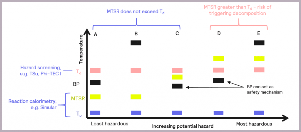
The schematic references the key reaction parameters introduced in Figure 5:

• the isothermal temperature of the reaction (T_p)
• the decomposition temperature of a component in the reaction mix (T_d)
• the Maximum Temperature of the Synthesis Reaction (MTSR)

It also introduces an additional parameter, the boiling point (BP) of the solvent or active chemicals used, as this is another factor that needs to be taken into account when considering the overall safety of a reaction. The relative order of these parameters in terms of temperature determines the criticality of the reaction.

• Scenario (A): the thermal order of the parameters is T_p<MTSR<BP<T_d. This represents the least hazardous reaction scenario, and no special measures are required as the MTSR does not exceed that of the BP of the solvent nor the T_d.
• Scenario (B): as with Scenario (A), the MTSR does not exceed T_d, although in this case, the BP of the solvent is higher than T_d (T_p<MTSR< T_d< BP). This means that, unlike Scenario (A), the BP will not act as a limit on the maximum temperature the reaction will attain, and heat accumulation conditions should be avoided.
• Scenario (C): the MTSR is higher than the BP but less than T_d (T_p< BP< MTSR<T_d). This means that risk reduction measures are required but that the BP of the solvent could be used as a non-ideal safety mechanism for the reaction.
• Scenario (D): the MTSR is higher than T_d, which means there is a risk that the decomposition could be triggered should the system fail. However, the BP of the solvent could be used as a limiting mechanism to prevent triggering the decomposition reaction, as BP is lower than T_d (T_p<BP<T_d<MTSR). In this case, risk reduction measures are required.
• Scenario (E): as with Scenario (D), the MTSR is greater than T_d, which means there is a risk that the decomposition could be triggered. However, the BP of the solvent is also above that of T_d, so it can’t be used as a safety barrier (T_p<T_d<MTSR<BP). In this case, emergency control measures are also required, which may include redesigning the process.

Although the Stoessel Diagram can help assess how hazardous a reaction is, caution needs to be exercised ​[3]​. For example, the solvent boiling point temperature assumes atmospheric pressure. Therefore, if the operating pressure becomes higher than this after a cooling failure, then the solvent boiling temperature also increases, effectively removing the safety mechanism in Scenario C and Scenario D. Similarly, if the solvent is rapidly vaporized by a fast energy release from decomposition, the reactor could become over-pressurized before the plant pressure relief mechanisms kick in. Therefore, while the Stoessel Diagram is useful to facilitate the development of intrinsically safer processes, it is important to recognize that a wider range of potential hazards must also be considered, pressure chief among them.

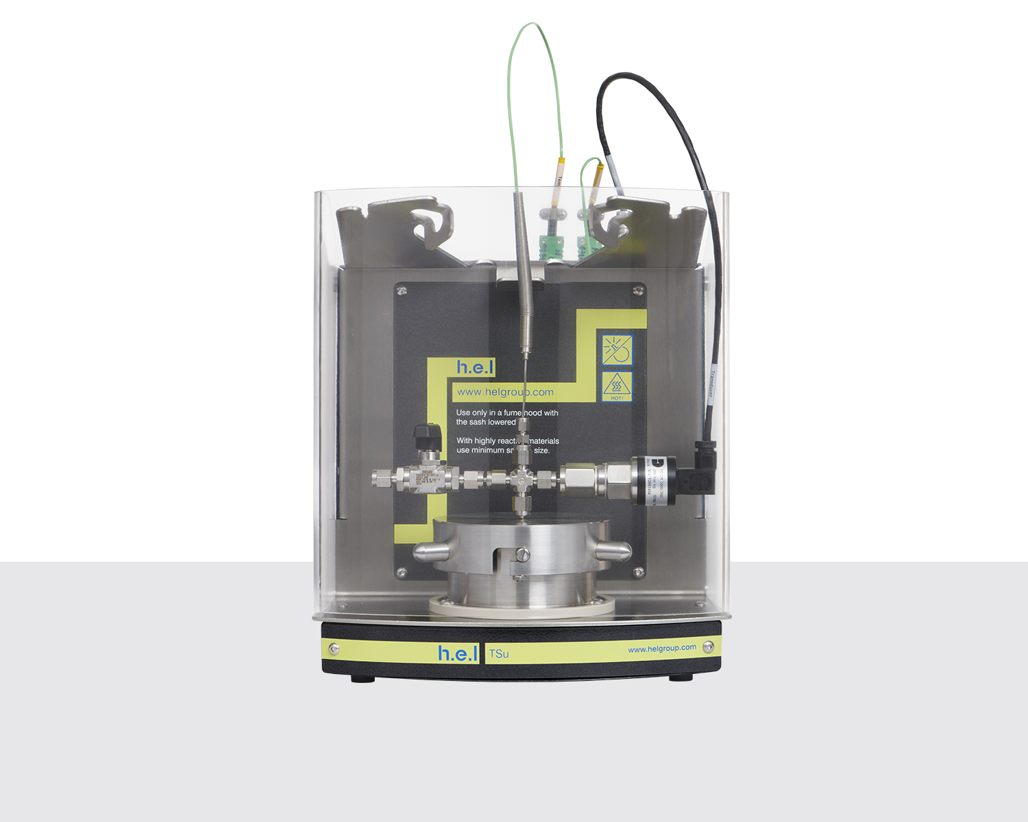
TSu | Thermal and Pressure Hazard Screening Platform

The fast screening of thermal and pressure hazards can be performed with the Thermal Scree...

Details

How Can The Operating Conditions Be Modified To Reduce The Risks Identified?

Stoessel diagrams can help us understand how risky chemical processes are, including desired reactions and secondary reactions (such as decomposition reactions). Stoessel classification identifies 5 possible scenarios, ranked from least dangerous to most dangerous. The commonality that the three first categories have, is that the maximum temperature of synthesis reaction (MTSR – the maximum temperature the reactor would reach if a failure in cooling occurs) stays under the temperature of decomposition (T_d, temperature at which some of the reactants or products start to break down at a detectable rate).In the case of scenarios (D) & (E), it is necessary to consider if the MTSR can be reduced by altering the conditions of the reaction to reduce the levels of accumulated reagent.

There are several ways this could be addressed, such as​ [1]​:

• Increasing the temperature of the reaction
• Increasing the pressure of the reaction
• Increasing the agitation of the reaction mix
• Adding a catalyst
• Reducing the feed rate of the reactant

The first four methods will increase the reaction rate and thus increase the reagent’s consumption rate. However, it must be balanced against the subsequent increase in the rate of heat evolved, and so an assessment on whether the plant’s cooling capacity can contain this increase in heat.

Reducing the reactants’ feed rate will reduce the reagent accumulation rate as it effectively allows more time for the reaction to occur and the rate-limiting reagent to be consumed before it accumulates to hazardous levels.

Exploring the impact of varying these different factors on the reaction is desirable. The Simular enables users to experiment in this way by creating experiments that facilitate the identification of optimum operating conditions for reducing thermal risk. For example, an esterification reaction in which acetic anhydride is fed into a reactor containing methanol can be kept at different temperatures. So let us analyze how different feed rates can affect the power needed to keep the conditions isothermal and accumulated reagent.

Reducing The Feed Rate

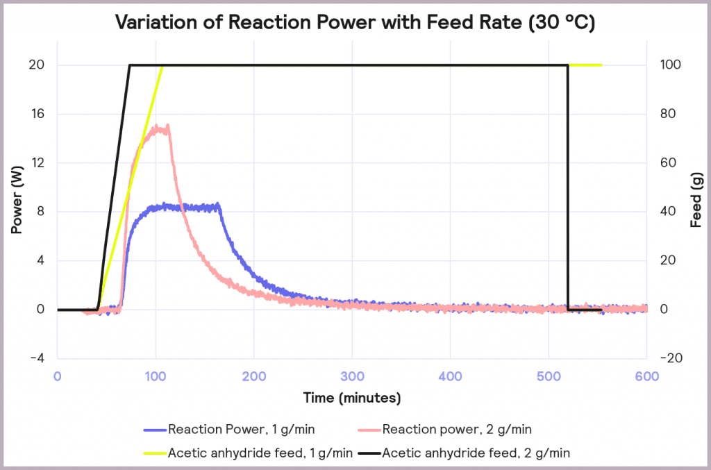
The effect of reducing the feed rate from 2 g/min to 1 g/min, while keeping the temperature of the process at 30 ⁰C, is illustrated in Figure 8.  It reduces the accumulation of reagent to 32% at the point at which the feed stops, and it reduces the maximum reaction power from 15 W to 8 W.  This reduction in maximum reaction power significantly reduces the cooling capacity required to keep the reaction isothermal and under thermal control.

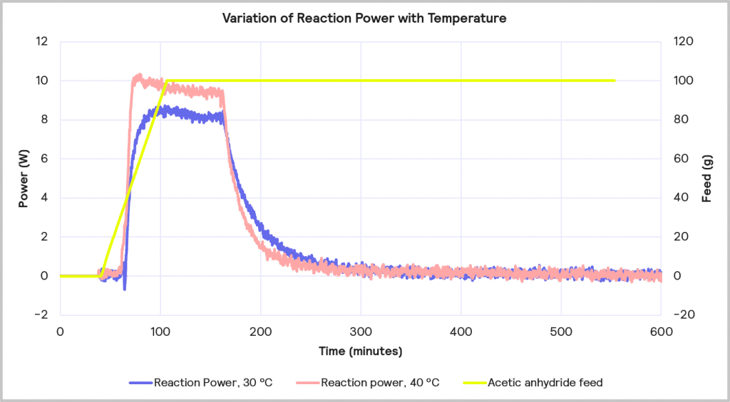
Increasing the Temperature

The accumulated reagent level can be further reduced by increasing the temperature from 30 ⁰C to 40 ⁰C while maintaining the slower feed rate of 1 g/min. The impact of this is depicted in Figure 11. This reduces the level of reagent accumulated to 22% at the point at which the feed is stopped, but it does increase the maximum reaction power from 8 W to 10 W.

Cooling Capacity Considerations

Increasing the reaction temperature poses an interesting question: while the increase in temperature will result in less accumulated reagent and thus a lower MTSR, should cooling fail, and a thermal runaway occurs, it does require a larger cooling capacity to deal with the faster rate of heat evolved. As before, if it is assumed that the 1 L lab-based reactor is initially scaling up to a 2000 L reactor, the 10W reaction power for the reaction run at 40⁰C equates to a 20 kW cooling capacity requirement on scale-up versus the 16 kW required for the same reaction run at 30⁰C. Therefore, although the 1g/min feed rate with 40⁰C process temperature is the desired combination from a safety point of view in terms of reagent accumulation, it may be that a lower temperature is required if the cooling capacity of the pilot plant is <20 kW.

Another vital consideration is the efficiency of the cooling. As the scale of the reaction increases, the thermal transfer efficiency from the temperature-controlling system will likely decrease. Because of this, the cooling capacity will probably have to increase. A suitable safety factor must also be applied to the cooling capacity to ensure the system can handle unexpected thermal events.

Ideally, a process should be as close to a dose-controlled reaction as possible. In this scenario, the reactant is consumed as rapidly as it is added. Therefore, in the event of a cooling or agitation failure, it is usually sufficient to switch off the feed to prevent a thermal runaway.

However, in cases where accumulation can’t be avoided, it is necessary to undertake a more detailed analysis of the risk.

Simular | Process Development Reaction Calorimeter

This highly configurable system from the H.E.L product family excels in optimizing process...

Details